A LOOK AT NYSE MARGIN DEBT AND THE MARKET

The New York Stock Exchange publishes end-of-month data for margin debt on the NYX data website, where we can also find historical data back to 1959. Let's examine the numbers and study the relationship between margin debt and the market, using the S&P 500 as the surrogate for the latter.

The first chart shows the two series in real terms — adjusted for inflation to today's dollar using the Consumer Price Index as the deflator. At the 1995 start date, we were well into the Boomer Bull Market that began in 1982 and approaching the start of the Tech Bubble that shaped investor sentiment during the second half of the decade. The astonishing surge in leverage in late 1999 peaked in March 2000, the same month that the S&P 500 hit its all-time daily high, although the highest monthly close for that year was five months later in August. A similar surge began in 2006, peaking in July 2007, three months before the market peak.

Debt hit a trough in February 2009, a month before the March market bottom. It then began another major cycle of increase.

The Latest Margin Data

The NYSE has released new data for margin debt, now available through May. The latest debt level is down 1.7% month-over-month. The May data gives us an additional sense of recent investor behavior.



At the suggestion of Mark Schofield, Managing Director at Strategic Value Capital Management, LLC, we've created the same chart with margin debt inverted so that we see the relationship between the two as a divergence.



The next chart shows the percentage growth of the two data series from the same 1995 starting date, again based on real (inflation-adjusted) data. We've added markers to show the precise monthly values and added callouts to show the month. Margin debt grew at a rate comparable to the market from 1995 to late summer of 2000 before soaring into the stratosphere. The two synchronized in their rate of contraction in early 2001. But with recovery after the Tech Crash, margin debt gradually returned to a growth rate closer to its former self in the second half of the 1990s rather than the more restrained real growth of the S&P 500. But by September of 2006, margin again went ballistic. It finally peaked in the summer of 2007, about three months before the market.



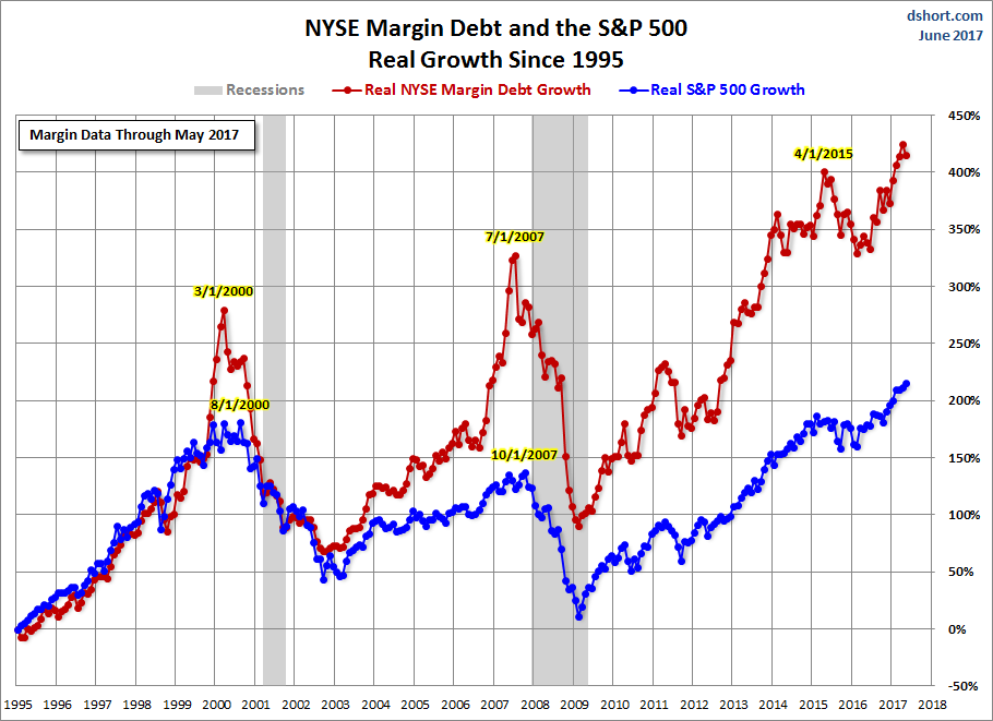
After the market low of 2009, margin debt again went on a tear until the contraction in late spring of 2010. The summer doldrums promptly ended when Chairman Bernanke hinted of more quantitative easing in his August 2010 Jackson Hole speech. The appetite for margin instantly returned, and the Fed periodically increased the easing. Even with QE now history, margin debt has reached another record high. The latest peak may not be a Fed-induced, easy-money bubble due to QE, but perhaps a response to the latest equity market rallies. It remains in high gear, as evidenced by the S&P 500 having logged over twenty record closes since the presidential election. For reference, last summer saw ten record closes and in November of 2014, there were twelve. As of this posting, the index is less than 1% below its latest record close.
NYSE Investor Credit

Lance Roberts of Real Investment Advice analyzes margin debt in the larger context that includes free cash accounts and credit balances in margin accounts. Essentially, he calculates the Credit Balance as the sum of Free Credit Cash Accounts and Credit Balances in Margin Accounts minus Margin Debt. The chart below illustrates the mathematics of Credit Balance with an overlay of the S&P 500. Note that the chart below is based on nominal data, not adjusted for inflation.



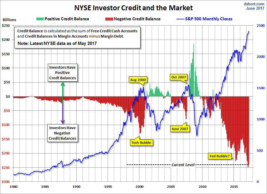
Here's a slightly closer look at the data, starting with 1995. Also, we've inverted the investor credit monthly data and used markers to pinpoint key turning points.



As we pointed out above, the NYSE margin debt data is several weeks old when it is published. Thus, even though it may, in theory, be a leading indicator, a major shift in margin debt isn't immediately evident. Nevertheless, we see that the troughs in the monthly net credit balance preceded peaks in the monthly S&P 500 closes by six months in 2000 and four months in 2007. The most recent S&P 500 correction greater than 15% was the 19.39% selloff in 2011 from April 29th to October 3rd. Investor Credit hit a negative extreme in March 2011.
Conclusions

There are too few peak/trough episodes in this overlay series to take the latest credit balance data as a leading indicator of a major selloff in U.S. equities. This has been an interesting indicator to watch in recent months and will certainly continue to bear close watching in the months ahead.

How Scared Is the Fed to Already Be Talking About QE Again?

Forget about normalization, the Fed is terrified.

The Fed officially began Quantitative Tightening in October. To date, the Fed has shrunk its balance sheet by less than $40 billion. And already Fed officials are so spooked by stocks falling, that they're promising more QE down the road… including an implicit purchasing of stocks.

To whit, on Friday, Boston Fed President Eric Rosengren stated the following:

If LSAPs (read: QE used to buy debt instruments) are indeed not effective, then the Fed may need to take other measures"

Let's be clear here... a major Fed official is implying the Fed should consider monetizing other assets, possibly even stocks... at a time when stocks are a mere 6% off ALL.TIME.HIGHS.

Just how vulnerable the US financial system that the Fed can't even stomach a NORMAL 10% correction without talking about QE again?

Let's be clear here. The Fed is terrified of the Everything Bubble bursting. And we're a lot closer to a crisis than most realize.

James Montier: The Advent of a Cynical Bubble

James Montier is one of my favorite market strategists. He is really good on behavioral economics. And his work inspired one of my favorite posts here on 17th century philosophers Descartes and Spinoza. James is also very good on his macro because he understands modern money and the sectoral balances framework of the late Wynne Godley.

Back during the financial crisis, James worked with Albert Edwards and Dylan Grice at French bank Societe Generale. And the three of them were a fearsome research trio. Unfortunately Dylan and James left the buyside. So Albert is holding down the fort at SocGen. And you can see what he's saying from some of my recent posts. 

But James has some new stuff out from his perch at fund manager GMO. That's the Boston-based fund manager whose G stands for founder Jeremy Grantham, whose market viewpoints I have detailed in the last few weeks. 

Extreme Overvaluation 

The title of James' last piece: The Advent of a Cynical Bubble. Here's the gist: 

That the US equity market is obscenely overvalued can hardly be news to anyone. Even a cursory glance at Exhibit 1 reveals that we are now at the second most expensive level of the Shiller P/E ever seen – surpassed only by the TMT bubble of the late 1990s! 

Only a handful of what we might call valuation deniers remain. They are dedicated to finding new and inventive ways to make equities look reasonable, and they have never yet met a bull market that they didn't love. 

So where Grantham was saying he was looking for a melt-up as confirmation of a bubble, James Montier is saying all indications are already there that we have a bubble. 

Managers are Overweight Equities 

He acknowledges that the Shiller P/E has its detractors. But it isn't the only metric showing extreme overvaluation in US equity markets. And survey data shows that fund managers know this. Yet, these same money managers are fully invested and overweight stocks. 

Source: GMO 

Now Grantham has said that the rest of the world offers relative value. And a chart from James clearly indicates this. The valuation differential is about the largest since the 1980s. 

Source: GMO 

But, these markets are not undervalued either. Look at India, for example. It's up 145% in 4 years and sports a 24x trailing multiple. That ain't cheap. 

Cynical? 

In the US, though, it's puzzling that everyone is fully invested. James calls it cynical. Everyone sees the overvaluation in stocks. But they act as if they believe they can get out before the bottom falls out. This will end badly though. Montier quotes Keynes to close his piece: 

It is the nature of organized investment markets, under the influence of purchasers largely ignorant of what they are buying and speculators who are more concerned with forecasting the next shift of market sentiment than with a reasonable estimate of future yield of capital – assets, that, when disillusion falls upon an over-optimistic and over-bought market, it should fall with sudden and catastrophic force. 

Caveat emptor.

Money and monetary stability in Europe, 1300-1914

There is a notable lack of long-run analyses of monetary systems and their stability. This column addresses this gap by looking at the monetary systems of major European states between 1300 and 1914. The evidence collected suggests that, despite many switches between standards and systems, fiscal capacity and political regimes ultimately shaped patterns of monetary stability. Theories of monetary stability that rely on the mechanics of monetary systems perform poorly when such a long-run perspective is taken.

In the literature on monetary systems, there are few empirical studies of the long run. Most long-run studies focus on the period after 1870 and the widespread adoption of the gold standard (e.g. Bordo and Rockoff 1996, Taylor 2002, Schularick and Taylor 2012). For the earlier period, Reinhart and Rogoff (2009) provide a comprehensive review of the historical evidence on monetary stability, and Allen (2001) and Pamuk and Özmucur (2002) provide data on price levels.

This is an important void, because only a long-run perspective can allow us to track the major transformations monetary systems went through, and to investigate the interplay between politics, technology, monetary institutions, and monetary outcomes. To help fill this void, in a recent study (Karman et al. 2018) we evaluated the long run patterns of monetary stability (defined as the stability of the monetary units in terms of silver/gold) and price stability (defined as the stability of the value of monetary units in terms of the goods basket).

Our study reveals that there was significant cross-country variation in monetary stability. While states in northwestern Europe stabilised their monetary units by the 17th and 18th centuries, states in eastern and southern Europe continued to depreciate them until the 20th century. Our study also shows that patterns of monetary stability shaped patterns of price stability. Thus explaining price stability requires explaining monetary stability. Finally, political variables emerge as the most important determinant of monetary stability. In particular, it was fiscally strong states with constraints on executive authority that ultimately stabilised the silver/gold value of their monetary units.

Monetary standards in history

Until the 20th century, the three widely adopted monetary standards were the silver, gold, and fiat standards.

On the silver standard, states set their monetary units equal to a certain weight of silver, and intrinsic value silver coins dominated the circulation. Silver standard was the most common standard in Europe until the 1870s.

On the gold standard, states set their monetary units equal to a certain weight of gold. Gold became the most common standard after the 1870s.

Finally, on the fiat standard, the silver/gold value of the monetary unit was left to float. Fiat standard evolved out of earlier experiments with ledger money (deposits that were transferable as book entries) and fiduciary money (copper coins and paper notes convertible to silver or gold on demand). States switched to the fiat standard when they suspended the convertibility of the fiduciary monies they issued. These suspensions could last anywhere from a few years to decades.

States continued to switch back and forth between silver, gold, and fiat standards until WWI.

Patterns of monetary stability

To track the patterns of monetary stability over time, we compiled the data on monetary standards and silver and gold equivalents of monetary units for England, Dutch Republic, France, Portugal, Spain, Austrian Habsburgs, Venice, Sweden, the Ottoman Empire, Poland-Lithuania, and Russia from 1300s to 1914.

Figure 1 The value of monetary unit, 1300-1914 (in grams of silver/gold)

Figure 1 gives an overview of the long-run patterns. For each monetary unit, the figure initially tracks the silver value (left axis) and later the gold value (right axis). The date the figure switches from tracking the silver value to gold value is marked with a dashed vertical line. Figure 1 also distinguishes between the periods the monetarysystem was on silver/gold standard (blue line) and fiat standard (red line).

First and foremost, Figure 1 establishes that states decreased the silver/gold value of their monetary units to ever lower levels over the centuries.

Second, it shows that states gradually changed the way they depreciated their monetary units against silver/gold. In the earlier periods, states depreciated their monetary units on the silver/gold standard by decreasing the silver or gold content of their intrinsic value coins (i.e. debasing their coinage). In later centuries, states depreciated their monetary units by switching to fiat standards and over-issuing fiat money.

Third, it shows that depreciations tended to be episodic. In particular, long periods of stability alternated with episodes when states depreciated their monetary units in consecutive years.

Fourth, there was a divergence in monetary stability across states. Western European states stabilised their monetary units relatively early, while states in southern and eastern Europe continued to depreciate them. On the other hand, there was no clear continent-wide historical break in stability associated with the introduction of a particular monetary technology or institution.

Figure 2 Index of the value of monetary unit, 1500-1914 (in silver/gold)

Notes: The index switches from tracking the value of monetary unit in silver to gold in 1717 for England, 1854 for Portugal, and 1870 for other states. Despite the different dates for the switch, because the market price ratio of gold to silver changed only from 10 to 15 from 1700s to 1870s, it had negligible impact on the overall patterns. Sweden, the most important copper producer in the continent, occasionally switched to copper standard and issued intrinsic value copper plates. We hold the index value for Sweden constant for those years.

Figure 2 also shows that most of the variation in monetary stability was not over time, but rather across states. The figure plots the value of the monetary unit first in terms of silver and later in terms of gold, normalising the index value in 1500 to one, correcting for the introductions of new monies and units, and putting all states in one figure. At one extreme, the Dutch Republic depreciated its monetary unit by about 2.3 times; at the other, the Ottomans depreciated by about 25,000 times. These patterns suggest country specific factors, rather than global or continent-wide shocks, shaped stability patterns.

Patterns of price stability

Next, we turn to patterns of price stability. Price stability concerns the stability of the value of the monetary unit in terms of the goods basket. The monetary unit could depreciate against the goods basket for two reasons. The first reason was that, as discussed in the previous section, states depreciated their monetary units against silver or gold. In other words, monetary instability caused price instability. The second reason was that silver or gold depreciated against the goods basket. In the early modern period, it was mainly inflows of precious metals from the New World that caused the depreciation of silver and gold against the goods basket. The empirical question is whether states' depreciation decisions or the silver/gold inflows from the New World had a greater role in driving price instability.

In Figure 3 we address this question. To keep the figure simple, it only covers the silver standard era (1500-1870). In the figure, the yellow area plots the price level; that is, the consumer price index in terms of the monetary unit of each state, normalised to 1 in year 1500. The figure also separates out the contributions of the two drivers of price inflation. The blue lines plot the depreciation of the monetary unit against silver (i.e. the contribution of monetary instability). The black lines plot the depreciation of silver against the goods basket.

David Stockman Exposes The Stock Market's $67 Trillion Nightmare

This is getting pretty ridiculous. For old times sake, we recently checked on the Federal debt level during the month we arrived in the Imperial City as a 24-year old eager beaver. That was June 1970 and the Federal debt held by the public was $275 billion.

Mind you, while that number wasn't exactly diminutive, it had taken all of 188 years to accumulate. That is to say, Uncle Sam had borrowed an average of $28,000 per week during the 9,776 weeks since George Washington was sworn in as the nation's first president.

We are ruminating about this seeming historical obscuranta because it just so happens that the US treasury this very week will be selling $258 billion of government debt.

That's right. Uncle Sam's scheduled debt emission this week will nearly equal his cumulative borrowing during the nation's first 188 years and its first 37 presidents!

And, yes, there has been some considerable inflation since June 1970. And not the least because exactly 13 months later Tricky Dick Nixon decided to pull the plug on Bretton Woods and the dollar's anchor to a fixed weight of gold.

Needless to say, the financial discipline of gold-backed money during that interval of guns and butter excess would most certainly have triggered a recession and a heap of inconvenience for Nixon's 1972 reelection prospects. As it happened, the American economy got a heap of inflation and destructive financialization over the next half century, instead.

Accordingly, the price level today is 5X higher as measured by the GDP deflator. So in today's dollars of purchasing power, the 1970 debt figure would be about $1.2 trillion.

This is by way of explaining that it hasn't been for nothing that we have labeled the Donald as the King of Debt and the Congressional Republicans as fiscal Benedict Arnolds. Their now enacted budget plan----which they have the gall to crow about from one end of the country to the other----is to borrow as much money in apples-to-apples dollars during the year ahead (FY 2019) as did the first 37 presidents of the United States!

Accordingly, Keynesians, beltway politicians of both parties and Wall Street punters, alike, know this: The US has a monumental debt problem, and it is most definitely not "priced-in".

So our purpose in this two-part series is to explain how it came to be not priced-in, and why that anomalous state of affairs is coming hard upon its sell-by date.

To be clear, we are not talking about just the $21 trillion of public debt that will be on the books after this week's borrowing binge, but the entire $67 trillion albatross of public and private debt that now strangles the US economy.

We refer to the latter as the lamentable outcome of the rolling national LBO that the US economy has undergone since June 1970.

The fact is, the $1.5 trillion of total public and private debt outstanding back then amounted to 150% of GDP. And that implicit 1.5X  national leverage ratio had essentially remained unchanged for the prior 100 years of robust economic growth and 25-fold rise in real income per capita.

By contrast, at $67 trillion of total debt today, the US leverage ratio stands at nearly 3.5X, and therein lies the giant financial skunk in the woodpile. Had the historically proven leverage ratio of 1.5X national income not been upended by Tricky Dick's perfidy, there would be $30 trillion of total debt on the US economy today, not $67 trillion.

So those two-extra turns of leverage amount to $37 trillion-----an economic millstone that is grinding capitalist growth steadily lower, and which has now put the main street and Wall Street economy alike in harm's way.

That's because the massive growth of central bank credit unleashed by the Camp David folly of 1971 has finally reached its limit---even by the lights of our overtly Keynesian central bankers. So they are now embarking upon an epochal balance sheet reversal that will drastically alter the fundamental dynamics of the financial system, and expose the vast falsification of financial asset values that are actually "priced-in" to today's Wall Street house of cards.

Indeed, it was today's Keynesian mind-frame that caused Nixon to jettison gold in the first place: He was advised by what we have called the "freshwater Keynesians" around Milton Friedman, who were every bit as statist on the matter of money and macro-economic management from Washington as were their "saltwater" compatriots in Cambridge, MA. They merely differed on technique as between monetary versus fiscal policy tools.

Alas, when practiced over a long enough time frame, however, Keynesians---and the politicians and apparatchiks who find it convenient to embrace their fatally flawed model---literally loose their minds. That is, insofar as historical memory is concerned.

Stated differently, they become incurably infected with "recency bias", and so doing end-up absolutely blind to the unsustainable errors and anomalies on which they whole debt-fueled scheme is predicted.

For instance, had your editor also checked in at the Eccles Building during his taxi ride from national airport to his new digs on Capitol Hill in June 1970, he would also have found that the Fed's balance sheet stood at a mere $55 billion. And that was after 56 years in the money printing business.

What happened during the next 48 years, of course, was nothing less than a monetary eruption----the very thing that Nixon's Camp David folly enabled. To wit, the Fed's balance sheet exploded by 82X or by nearly 10% per annum over the course of a half century.

It goes without saying that you could not have found one economist (or even layman) in Washington, Cambridge or Chicago in June 1970 who would have recommended or even imagined an 82X explosion of the central banks balance sheet during the next 50 years. Even the reining monetary populist and crackpot of the day, Congressman Wright Patman of Texas and Chairman of the House banking and currency committee, would have never countenanced such a thing.

The rest is history, of course, and it couldn't have been imagined, either.That is, the 82Xexplosion of central bank credit gave rise to the freakish chart below.

To wit, in June 1970 the GDP was $1.1 trillion and it has since expanded by 18X to $19.6 trillion. By contrast, total public and private debt outstanding was $1.58 trillion and has since expanded by 42X to $67 trillion.

Needless to say, to grow these unsustainably divergent trends for even another decade would lead to an outright absurdity. To wit, $35 trillion of nominal GDP and $150 trillion of total debt.

In fact, the ridiculousness of it perhaps explains why the Fed stopped publishing the total credit market debt figure in its quarterly "Flow of Funds" report in Q4 2015 when the number stood at $63.5 trillion. But the components are still there and they do add to $67 trillion.

Needless to say, this chart makes all the difference in the world for the impending era of interest rate normalization and quantitative tightening (QT). It is one thing to permit interest rates to rise by 200-300 basis points in a context when the economy is carrying $30 trillion of debt; it's an altogether different kettle of fish, of course, when the burden is $67 trillion.

In short, recency bias is going to prove to be the Achilles heel of the now ending era of Bubble Finance. The US economy has been borrowing and printing money so long that its position on the economic and financial map has been lost sight of---meaning that the impact of the coming epochal reversal at the central bank is not even remotely appreciated.

Take the matter of the Fed's balance sheet. Even had the US followed Milton Friedman's fixed money growth rule at approximately 3% per annum, the Fed's $55 billion balance sheet of June 1970 would stand at just $230 billion today.

Do we think that $4.2 trillion of extra central bank credit has changed everything?

Yes, we do---as we will amplify in Part 2.

In the interim, however, here is the singular chart that should scare the bejesus out of casino gamblers who remain drunk on the trading charts embedded in robo-machines and the fancy bespoke trades peddled by Wall Street brokers.

Up to $2 trillion of central bank balance sheet shrinkage has never happened before. Nor has the impact been any more imagined at present than had been the 82X explosion of the Fed's balance sheet back in June 1970.